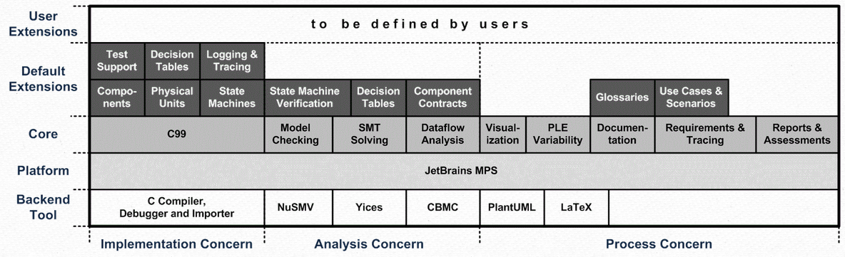
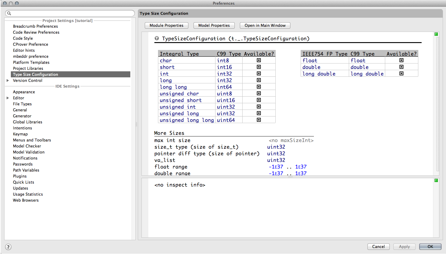
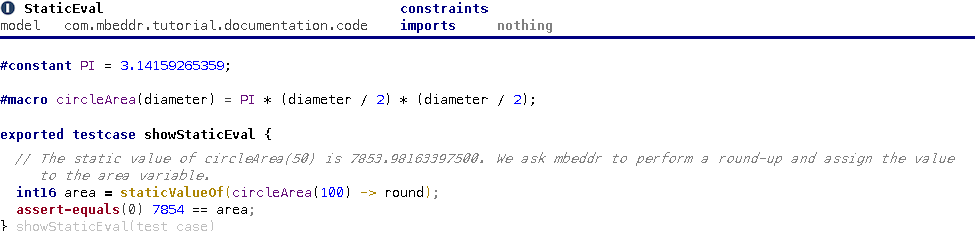
7.2 Units
The purpose of physical units is to annotate types and literals with additional information - units - used to improve type checking. Many embedded systems work with real-world quantities, and many of those have a physical unit associated with them.
7.2.1 Physical Units Basics
Defining and Attaching Units to Types Let us go back to the definition of Trackpoint introduced in Section Function Pointers and make it more useful. Our application is supposed to work with tracking data (captured from a bike computer or a flight logger). For the examples so far we were not interested in the physical units.
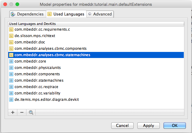
Let us now explore how we can work with physical units, adding more semantics to this data structure. In order to use the physical units language, we need to import either the com.mbeddr.physicalunits devkit. After the import we can add units for the types by simply pressing the / at the right side of them.
The 7 standard SI units are available from an accessory module called SIUnits. It can be imported into any implementation module. There is an extra nounit unit defined in this module. The usage of this unit is limited to test case definitions and conversion rules, which we will talk about in later sections. When you import this module, the simple units like s and m will be immediately available.
For the speed member of the Trackpoint struct we need to add m/s. Since this is not an SI base unit, we first have to define it, which can be done either in the ImplementationModule or in a UnitContainer (such as UnitDeclarations). To create a new unit just use its alias unit. The specification of the derived units can be typed in after the name of the unit. A simple unit specification consists of one unit with possibly an exponent. If you would like to type in a composite unit specification then press ENTER to expand the components in the specifiction. Exponents can be added to the units by pressing the cap (^) symbol and the value of the exponent. This works for all units in the specification except for the last component; there the cap is disabled because it conflicts with the binary XOR operator. At the last position use the appropriate intention (by the way it is available for all components regardless of the position in the specification) to add the exponent to the unit. An exponent can either be simple integer number or it can be transformed to a fraction by typing / in the exponent expression.
The following code example shows how can we use units for the members of the Trackpoint struct.
exported struct Trackpoint {

  int8 id;

  int8/s/ time;

  int8/m/ x;

  int8/m/ y;

  int16/m/ alt;

  int16/mps/ speed;

};
Units on Literals Adding these units may result in errors in the existing code (depending on whether you had added them in previous tutorial steps) because you cannot simply assign a plain number to a variable or member whose type includes a physical unit (int8/m/ length = 3; is illegal). Instead you have to add units to the literals as well. You can simply type the unit name after the literal to get to the following:
Trackpoint i1 = {
id = 1,
time = 0 s,
x = 0 m,
y = 0 m,
alt = 100 m
};
You also have to add them to the comparison in the assertions as well, for example in this one:
{

  processor = :process_doNothing;

  Trackpoint i2 = processor(i1);

  assert(0) i2.id == 1 && i2.alt == 100 m;

}
Operators If we were to write the following code, we would get an error:
int8 someInt = i1.x + i1.speed; // error, adding m and mps
This is because all the mathematical operators are overloaded for physical units and these operations are also type-checked accordingly. Clearly, the problem with this code is that you cannot add a length (i1.x) and a speed (i1.speed). The result is certainly not a plain int8, so you cannot assign the result to someInt. Adding i1.x and i1.y will work, though. Another example where the units are matched properly:
int8/mps/ speed1 = (i4.x - i3.x) / (i4.time - i3.time);
The calcVerticalSpeed provides a few more examples of working with units in expressions:
void calcVerticalSpeed(TrackpointWithVertical* prev, TrackpointWithVertical* cur) {
/* cur.alt = 0 m; */
/* cur.speed = 0 mps; */
if (prev == null) {
cur.vSpeed = 0 mps;
} else {
int16/m/ dAlt = cur.alt - prev.alt;
int8/s/ dTime = cur.time - prev.time;
cur.vSpeed = dAlt / dTime;
}
} calcVerticalSpeed (function)
Editing Composite Units When you edit an expression with composite units you may encounter the problem that multiple side transformations are available at a given place and so you need to make the choice by hand. Consider the following code example:
int8/mps/ speed2 = 2 m・s-1 + 3 s-1・m;
Here, when you are editing the unit definition of the number literal 2, the * operator may be used at the end to introduce a multiplication in the expression or to extend the unit defition. Similarly, the ^ symbol may be used to introduce exponent for the units or could be also used for the binary xor operator. This problem only arises at the end of the unit definition.
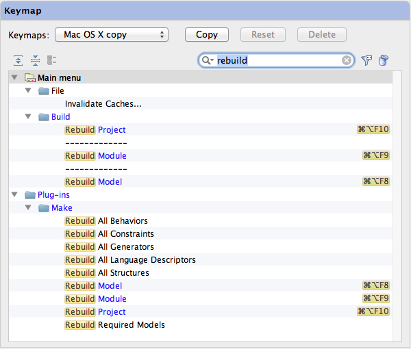
Build Configuration If you try to rebuild the model, you will get an error message, saying that you need to add the units configuration item to the build configuration. If you have added this item, the build should be successful and we should be able to run the test again.
7.2.2 Unit Conversions
So far, we have used units only for type checking. However, sometimes you have several units for the same physical quantity. For example, speed can be measured in m/s or km/h. For this purpose you can define conversion rules between the units.
Defining Conversions The conversion rule must define a source and a target unit (the conversion will happen between these units) and it must contain one or more conversion specifiers. A conversion specifier defines the conversion expression for a given type. Inside the conversion expression one can use the val expression as a placeholder for the to-be-converted value. It will be substituted with the value that is passed to the conversion rule. The type that you define for the specifier is the type that the val expression will have. Additionally, it is also possible to omit the type: in this case the specifier works as a generic one, where the expression may be applied to any types (the type of the val expression will be double in this case, but this is just a trick that is needed for the typesystem to work properly). The conversion specifiers are checked, and redundant specifiers will be marked as erroneous (the ones that are covered by some other specifier due to its type being the supertype of the original type).
section conversions {
exported conversion mps -> kmh {
exported conversion kmh -> mps {
exported conversion s -> h {
exported conversion m -> km {
} section conversions
val as double -> val * 3.6 val as <no type> -> val / 3.6 val as <no type> -> val / 3600 val as <no type> -> val / 1000
} } } }
Conversion rules can be either lazy or eager. The default behavior is the lazy evaluation, you can switch to eager from the corresponding intention on the conversion rule itself.
-
Lazy conversion rule: the val expression inside the conversion specifier has no unit, and the expression must evaluate to a type without units. During the usage of the conversion rule, the type system will just simply append the rule's target unit to the evaluated expression.
-
Eager conversion rule: the val expression has the same unit as the rule's source unit. The expression in the conversion specifier must evaluate to a type with the rule's target unit. During the usage of the conversion rule, the expression will be simply evaluated and the resulting type will be used (which must match the target unit).
Using Conversions You can now invoke this conversion within a convert expression:
void somethingWithConversion() {
Trackpoint highSpeed;
highSpeed.speed = ((int16/mps/) convert[300 kmh-> mps]);
} somethingWithConversion (function)
The convert expression does not explicitly refer to any specific conversion rule, you only need to define the target unit of the conversion, while the source unit is known from the type of the original expression. The system will try to find a matching conversion specifier (where both the units and the types match). Here comes the conversion specifier with no specific type handy, because it can be applied to any expression if the units match.
The conversion specifier can be set manually too in the Inspector of the convert expression.
7.2.3 Generic Units
Generic units can be used to enhance the type safety for function calls by also providing the possibility to specify the function in a generic way with respect to the used type annotations. The following code snippets show some use cases of generic units:
int8/U1/ sum(int8/U1/ a, int8/U1/ b) {
return a + b;
} sum (function)
int8/U1・U2/ mul(int8/U1/ a, int8/U2/ b) {
return a * b;
} mul (function)
Trackpoint process_generic(Trackpoint e) {
e.time = sum(10 s, 10 s);
e.id = sum(1, 2);
e.x = sum(10 m, 10 m);
e.speed = mul(10 m, 10 s-1);
return e;
} process_generic (function)
First you need to create generic units by invoking the Add Generic Unit Declaration intention on the function. You can specify multiple generic units once the first one has been created by just simply pressing Enter in the unit list. These newly created generic units can then be used for the type annotation just like any other unit. The substitutions will be computed based on the input parameters of the function call. One can also combine a generic unit with additional arbitrary non-generic units for the type annotations of the parameters and the return type. In addition, it is also possible to invoke the function with bare types, but be aware that once at least one substitution is present, the function call will be type checked also for matching units. The generic units can also have exponents (even as fractions) and the same type-checks also apply to them as it was described for the non-generic units. An example shows how this could be done for a square root function:
double/U112/ sqrt(double/U1/ a) {
double/U112/ res = 0 U112;
//here goes your sophisticated square root approximation
return res;
} sqrt (function)
Some additional notes on the usage of the generic units:
- You should not use multiple generic units in the annotation of one given function parameter, because the non-generic units will be bound to the first generic unit (all of them), so the substitutions will probably not be the ones that you would expect. This is a constraint introduced to manage the complexity of the compuatation of the bindings; allowing multiple generic units for parameter types could result in a constraint solving problem which we do not support right now.
- The generic units can only be used inside the function definition, this means that they are not visible outside of the function definition.
7.2.4 Stripping and Reintroducing Units
Let us assume we have an existing (legacy or external) function that does not know about physial units and you cannot or do not want to use generic units. An example is anExistingFunction:
int16 anExistingFunction(int16 x) {
return x + 10;
} anExistingFunction (function)
To be able to call this function with arguments that have units, we have to strip away the units before we call the function. This can be achieved by selecting the corresponding expression and invoking the Strip Unit intention. The type of this stripped expression will be simply the type of the original expression but without units.
int16/m/ someFunction(Trackpoint* p1, Trackpoint* p2) {
int16 newValueWithoutUnit = anExistingFunction(stripunit[p1.alt]);
return newValueWithoutUnit m;
} someFunction (function)
The opposite direction (i.e., adding a unit to a value that has no unit) is also supported. The introduceunit operator is available for this. It takes an expression plus the to-be-introduced unit as arguments.
7.3 State Machines
Next to components and units, state machines are one of the main C extensions available in mbeddr. They can be used directly in C programs, or alternatively, embedded into components. To keep the overall complexity of the example manageable, we will show how state machines can be used directly in C.
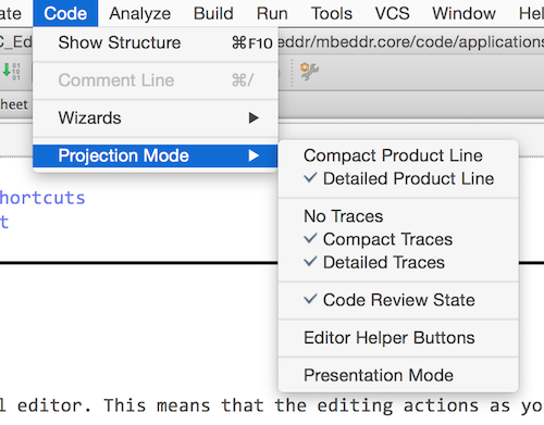
State machines can either be viewed and edited with the textual notation or with the table based projection. You can switch between the two modes with the option.
This section will give a brief overview on state machines; how they can be defined, how one could interact with C code when using the state machines and we will also give details about hierarchical state machines and their visualizations with the help of the PlantUML tool.
7.3.1 Implementing a State machine
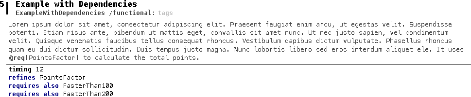
Import the com.mbeddr.statemachines devkit into your model and create a new ImplementationModule (the example module is called also StateMachines. Then you can create the state machine in this module and add the ImplementationModule to the build configuration. This section will guide you through an example that creates a state machine for a flight judgement system. This system has 5 states which describe the behavior of the plane and also give the semantics for awarding the points for a given flight. We will create these states and see how they can be connected with transitions. We will also explore how one could specify guard conditions for the transitions. The informal rules for judging flights are as follows:
- Once a flight lifts off, you get 100 points
- For each trackpoint where you go more than 100 mps, you get 10 points
- For each trackpoint where you go more than 200 mps, you get 20 points
- You should land as short as possible; for each trackpoint where you are on the ground, rolling, you get 1 point deducted.
- Once you land successfully, you get another 100 points.
In order to create the state machine in the ImplementationModule simply type in statemachine at the top level in implementation modules. This will create a new state machine with an initial state and one event already defined. You can leave the event there, we will come back to that later. We know that the airplane will be in various states: beforeFlight, airborne, landing (and still rolling), landed and crashed. You can just rename the already existing initial state to beforeFlight and add the other states to the state machine. In the end you should have the following states:
exported statemachine FlightAnalyzer initial = beforeFlight {
state beforeFlight {
} state beforeFlight
state airborne {
} state airborne
state landing {
} state landing
state landed {
} state landed
state crashed {
} state crashed
}
The state machine will accept two kinds of events. The first one is the next event, which takes the next trackpoint submitted for evaluation. Note how an event can have arguments of arbitrary C types, a pointer to a Trackpoint in this example. The Trackpoint struct is already defined in the DataStructures module. The other event, reset, resets the state machine back to its initial state.
exported statemachine FlightAnalyzer initial = beforeFlight {
in event next(Trackpoint* tp) <no binding>
in event reset() <no binding>
}
We also need a variable in the state machine to keep track of the points we have accumulated during the flight. In order to create a new variable simply type var in the state machine. This creates a new variable, you need to specify its name and the type. The newly created variable is invisible from outside by default, you can change this to readable or writable with the corresponding intentions. Readable variables may be read from outside of the state machine, while writable variables can also be modified from the interacting C code (you will have to create a state machine instance first; we explain this below). In the end you should have a points variable in the state machine which is readable only:
exported statemachine FlightAnalyzer initial = beforeFlight {
readable var int16 points = 0
}
We can now implement the rules outlined above using transitions and actions. Let us start with some simple ones. Whenever we enter beforeFlight we reset the points to 0. We can achieve this with an entry action in beforeFlight:
exported statemachine FlightAnalyzer initial = beforeFlight {
state beforeFlight {
entry { points = 0; }
} state beforeFlight
}
There are some additional rules for taking off, landing and conditions for crashing.
-
All states other than beforeFlight must have a transition triggered by the reset event to go back to the beforeFlight state. Note, that as a consequence of the entry action in the beforeFlight state, the points get reset in all three cases.
-
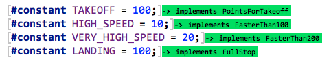
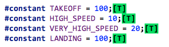
As soon as we submit a trackpoint where the altitude is greater than zero we can transition to the airborne state. This means we have successfully taken off, and we should get 100 points in bonus. TAKEOFF is a global constant representing 100 (
#constant TAKEOFF = 100;). We also make use of the physical units extension (see Section Units) and annotate the speed and altitude with the appropriate unit.
-
Events while we are in the air: when we are airborne and we receive a trackpoint with zero altitude and zero speed (without going through an orderly landing process), we have crashed. If we are at altitude zero with a speed greater than zero, we are in the process of landing. The other two cases deal with flying at over 200 and over 100 mps. In this case we stay in the airborne state (by transitioning to itself) but we increase the points.
The complete set of transitions is as follows:
exported statemachine FlightAnalyzer initial = beforeFlight {
state beforeFlight {
entry { points = 0; }
on next [tp.alt > 0 m] -> airborne
exit { points += TAKEOFF; }
} state beforeFlight
state airborne {
on next [tp.alt == 0 m&& tp.speed == 0 mps] -> crashed
on next [tp.alt == 0 m&& tp.speed > 0 mps] -> landing
on next [tp.speed > 200 mps&& tp.alt == 0 m] -> airborne { points += VERY_HIGH_SPEED; }
on next [tp.speed > 100 mps&& tp.speed <= 200 mps&& tp.alt == 0 m] -> airborne { points += HIGH_SPEED; }
on reset [ ] -> beforeFlight
} state airborne
state landing {
on next [tp.speed == 0 mps] -> landed
on next [tp.speed > 0 mps] -> landing { points--; }
on reset [ ] -> beforeFlight
} state landing
state landed {
entry { points += LANDING; }
on reset [ ] -> beforeFlight
} state landed
state crashed {
entry { send crashNotification(); }
} state crashed
}
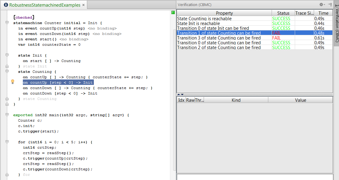
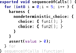
Note that the transitions are checked in the order of their appearance in the state machine; if several of them are ready to fire (based on the received event and the evaluation of the guard conditions), the first one is picked. Actually this kind of nondeterminism is usually not wanted and mbeddr provides support for the verification of state machines, which you can read more about in Section Checking State Machines.
Junction states (influenced by Simulink) can also be created in the state machine in mbeddr. A junction state can only contain epsilon-transitions, meaning these transitions are immediately ready to fire when the state is entered, they don't need a triggering event. Having multiple epsilon-transitions clearly introduces nondeterminism, so one typically specifies guards for these transitions. The following example uses the points variable to select the state transition that should be applied. The example junction state makes a decision based on the points and immediately fires.
exported statemachine FlightAnalyzer initial = beforeFlight {
junction NextRound {
[points > 100] -> airborne
[points <= 100] -> beforeFlight
} junction NextRound
}
Junctions are essentially branching points in a statemachine and help modularize complex guards (especially if several guards in one state have common subexpressions):
7.3.2 Interacting with Other Code -- Outbound
So how do we deal with the crashed state? Assume this flight analyzer runs on a server, analyzing flights that are submitted via the web. If we detect a crash, we want to send notifications or perform other kinds of error handling. In any case, this would involve the invocation of some external code. This can be performed in two ways:
The first one is to simply invoke a C function from an entry or exit action. Another alternative, which is more suitable for formal analysis (as we will see below and in Section Checking State Machines) involves out events. From the entry action we send an out event, which we have defined in the state machine. The following code example shows how the latter one would look like.
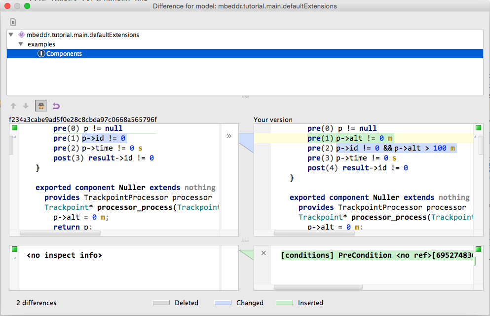
StateMachines
model mbeddr.tutorial.main.defaultExtensions
package examples constraints
exported statemachine FlightAnalyzer initial = beforeFlight {
out event crashNotification() => raiseAlarm
state crashed {
entry { send crashNotification(); }
} state crashed
}
void raiseAlarm() {
//invoke some kind of real-world thingy
//that reacts suitably to a detected crash
} raiseAlarm (function)
imports FlightJudgementRules
DataStructures
stdlib_stub
stdio_stub
UnitDeclarations
SIUnits
We create an out event called crashNotification (which will be sent when we enter the crashed state). We then specify a binding to the out event; the binding is part of the out event definition: simply add the name of the function as the target of the arrow (in the example this is the raiseAlarm function).
The benefit of this approach compared to the previous one is that formal verification can check whether the notification was sent at all during the execution of the state machine. The effect is the best of both worlds: in the generated code we do call the raiseAlarm function, but on the state machine level we have abstracted the implementation from the intent. See Section Checking State Machines for a discussion of state machine verification.
7.3.3 Interaction with Other Code -- Inbound
Let us write some test code that interacts with a state machine. To write a meaningful test, we will have to create a whole lot of trackpoints. So to do this we create helper functions. These in turn need malloc and free, so we first create an additional external module that represents stdlib.h:
stdlib_stub
// contents are exported by default
model com.mbeddr.tutorial.documentation.code imports nothing
void* malloc(size_t size);
void free(void* ptr);
resources header: <stdlib.h>
We can now create a helper function that creates a new Trackpoint based on an altitude and speed passed in as arguments:
exported Trackpoint* makeTP(int16 alt, int16 speed) {
static int8 trackpointCounter = 0;
trackpointCounter++;
Trackpoint* tp = ((Trackpoint*) malloc(sizeof[Trackpoint]));
tp.id = trackpointCounter;
tp.time = trackpointCounter s;
tp.alt = alt m;
tp.speed = speed mps;
return tp;
} makeTP (function)
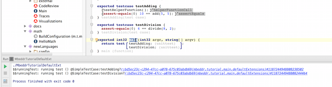
We can now start writing (and running!) the test. We first create an instance of the state machine (state machines act as types and must be instantiated). We then initialize the state machine by using the init operation:
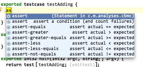
exported testcase testFlightAnalyzer {
FlightAnalyzer f;
f.init;
assert(0) f.isInState(beforeFlight);
assert(1) f.points == 0;
f.trigger(next|makeTP(0, 20));
assert(2) f.isInState(beforeFlight) && f.points == 0;
f.trigger(next|makeTP(100, 100));
assert(3) f.isInState(airborne) && f.points == 100;
test statemachine f {
next(makeTP(200, 100)) ➔ airborne
next(makeTP(300, 150)) ➔ airborne
next(makeTP(0, 90)) ➔ landing
next(makeTP(0, 0)) ➔ landed
}
assert-equals(4) f.points == 200;
} testFlightAnalyzer(test case)
Initially we should be in the beforeFlight state. We can check this with an assertion:
exported testcase testFlightAnalyzer {
f.init;
assert(0) f.isInState(beforeFlight);
assert(1) f.points == 0;
f.trigger(next|makeTP(0, 20));
assert(2) f.isInState(beforeFlight) && f.points == 0;
f.trigger(next|makeTP(100, 100));
assert(3) f.isInState(airborne) && f.points == 100;
test statemachine f {
next(makeTP(200, 100)) ➔ airborne
next(makeTP(300, 150)) ➔ airborne
next(makeTP(0, 90)) ➔ landing
next(makeTP(0, 0)) ➔ landed
}
assert-equals(4) f.points == 200;
} testFlightAnalyzer(test case)
We also want to make sure that the value of points is zero initially. Since we have declared the points variable to be writable above, we can write:
exported testcase testFlightAnalyzer {
f.init;
assert(0) f.isInState(beforeFlight);
assert(1) f.points == 0;
f.trigger(next|makeTP(0, 20));
assert(2) f.isInState(beforeFlight) && f.points == 0;
f.trigger(next|makeTP(100, 100));
assert(3) f.isInState(airborne) && f.points == 100;
test statemachine f {
next(makeTP(200, 100)) ➔ airborne
next(makeTP(300, 150)) ➔ airborne
next(makeTP(0, 90)) ➔ landing
next(makeTP(0, 0)) ➔ landed
}
assert-equals(4) f.points == 200;
} testFlightAnalyzer(test case)
Let us now create the first trackpoint and pass it in. This one has speed, but no altitude, so we are in the take-off run. We assume that we remain in the beforeFlight state and that we still have 0 points. Notice how we use the trigger operation on the state machine instance. It takes the event as well as its arguments (if any):
exported testcase testFlightAnalyzer {
f.init;
assert(0) f.isInState(beforeFlight);
assert(1) f.points == 0;
f.trigger(next|makeTP(0, 20));
assert(2) f.isInState(beforeFlight) && f.points == 0;
f.trigger(next|makeTP(100, 100));
assert(3) f.isInState(airborne) && f.points == 100;
test statemachine f {
next(makeTP(200, 100)) ➔ airborne
next(makeTP(300, 150)) ➔ airborne
next(makeTP(0, 90)) ➔ landing
next(makeTP(0, 0)) ➔ landed
}
assert-equals(4) f.points == 200;
} testFlightAnalyzer(test case)
Now we lift off by setting the alt to 100 meters:
exported testcase testFlightAnalyzer {
f.init;
assert(0) f.isInState(beforeFlight);
assert(1) f.points == 0;
f.trigger(next|makeTP(0, 20));
assert(2) f.isInState(beforeFlight) && f.points == 0;
f.trigger(next|makeTP(100, 100));
assert(3) f.isInState(airborne) && f.points == 100;
test statemachine f {
next(makeTP(200, 100)) ➔ airborne
next(makeTP(300, 150)) ➔ airborne
next(makeTP(0, 90)) ➔ landing
next(makeTP(0, 0)) ➔ landed
}
assert-equals(4) f.points == 200;
} testFlightAnalyzer(test case)
So as you can see it is easy to interact from regular C code with a state machine. For testing, we have special support that checks if the state machine transitions to the desired state if a specific event is triggered. Here is some example code (note that you can use the test statemachine construct only within test cases):
exported testcase testFlightAnalyzer {
f.init;
assert(0) f.isInState(beforeFlight);
assert(1) f.points == 0;
f.trigger(next|makeTP(0, 20));
assert(2) f.isInState(beforeFlight) && f.points == 0;
f.trigger(next|makeTP(100, 100));
assert(3) f.isInState(airborne) && f.points == 100;
test statemachine f {
next(makeTP(200, 100)) ➔ airborne
next(makeTP(300, 150)) ➔ airborne
next(makeTP(0, 90)) ➔ landing
next(makeTP(0, 0)) ➔ landed
}
assert-equals(4) f.points == 200;
} testFlightAnalyzer(test case)
You may have noticed that the helper function allocates the new Trackpoints on the heap, without releasing the memory. You could simply call free on these newly created structures after the test statement has been executed or allocate the trackpoints on the stack to solve this problem.
7.3.4 Hierarchical State Machines
State machines can also be hierarchical. This means that a state may contain essentially a sub-state machine. The following piece of code shows an example. It was derived from the previous flight judgement example, but the three flying, landing and landed states are now nested inside the airborne composite state. Composite states can be created in the state machine by typing composite state.
exported statemachine HierarchicalFlightAnalyzer initial = beforeFlight {
macro stopped(next) = tp.speed == 0 mps
macro onTheGround(next) = tp.alt == 0 m
in event next(Trackpoint* tp) <no binding>
in event reset() <no binding>
out event crashNotification() => raiseAlarm
readable var int16 points = 0
state beforeFlight {
entry { points = 0; }
on next [tp.alt > 0 m] -> airborne
exit { points += TAKEOFF; }
} state beforeFlight
composite state airborne initial = flying {
on reset [ ] -> beforeFlight { points = 0; }
on next [onTheGround && stopped] -> crashed
state flying (airborne.flying) {
on next [onTheGround && tp.speed > 0 mps] -> landing
on next [tp.speed > 200 mps] -> flying { points += VERY_HIGH_SPEED; }
on next [tp.speed > 100 mps] -> flying { points += HIGH_SPEED; }
} state flying
state landing (airborne.landing) {
on next [stopped] -> landed
on next [ ] -> landing { points--; }
} state landing
state landed (airborne.landed) {
entry { points += LANDING; }
} state landed
} state airborne
state crashed {
entry { send crashNotification(); }
} state crashed
}
Here are the semantics:
- When a transition from outside a composite state targets a composite state, the initial state in that composite state is activated.
- A composite state can have its own transitions. These act as if they were defined for each of the states of the composite state.
-
If a transition from an inner state
A crosses a composite state-boundary B, then the actions happen in the following order: exit actions of A, exit actions of B, transition action, and entry action of the transition's target (which is outside of the composite state).
7.3.5 Tabular Notation
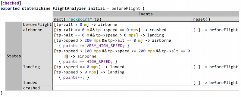
State machines can also be rendered and edited as a table: the events become the column headers, and the states become the row headers. Fig. 7.3.5-A shows an example. You can switch projection modes the usual way via the .
Figure
7.3.5-A: The FlightAnalyzer state machine shown as a table.
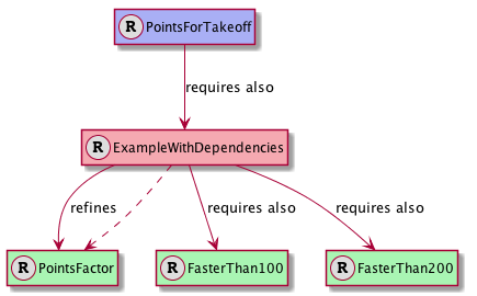
7.3.6 State Machine Diagrams
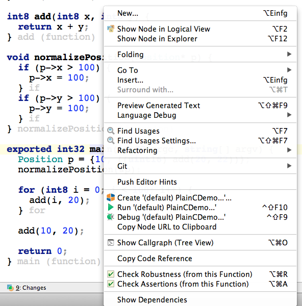
State machines can also be visualized with PlantUML (a graphical editor will be done soon). The visualization can be generated from the context menu of the state machine. You may want to use the statechart or statechart (short), the former one displays all information for the transitions while the latter one will only print the event's name which triggers the given transition.
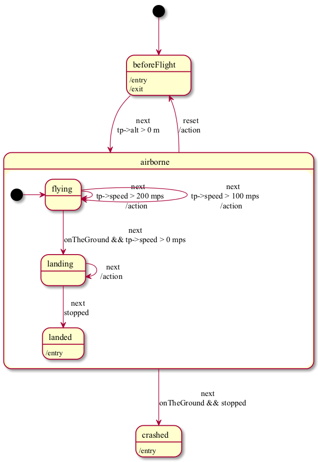
Fig. 7.3.6-A shows an example visualization for the hierarchical state machine that was described in the previous section.
Figure
7.3.6-A: A visualization of a state machine in mbeddr. You can click on the states and transitions to select the respective element in the editor.
7.4 Components
Let us now introduce components to further structure the system. We start by factoring the Trackpoint data structure into a separate module and export it to make it accessible from importing modules.
exported struct Trackpoint {
int8 id;
int8/s/ time;
int8/m/ x;
int8/m/ y;
int16/m/ alt;
int16/mps/ speed;
};
7.4.1 An Interface with Contracts
We now define an interface that processes Trackpoints. To be able to do that we have to add the com.mbeddr.components devkit to the current model. We can then enter a client-server interface in a new module Components. We use pointers for the trackpoints here to optimize performance. Note that you can just press * on the right side of Trackpoint to make it a Trackpoint*.
The interface has one operation process.
exported cs interface TrackpointProcessor {
Trackpoint* process(Trackpoint* p)
}
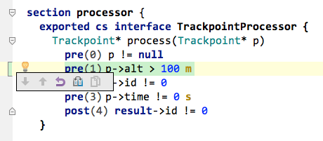
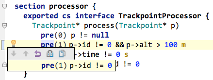
To enhance the semantic "richness" of the interface we add preconditions and a postcondition. To do so, use an intention on the operation itself. Please add the following pre- and postconditions (note how you can of course use units in the precondition). The result expression is only available in postconditions and represents the result of the executed operation.
exported cs interface TrackpointProcessor {
Trackpoint* process(Trackpoint* p)
pre(0) p != null
pre(1) p.id != 0
pre(2) p.time != 0 s
post(3) result.id != 0
}
After you have added these contracts, you will get an error message on the interface. The problem is this: if a contract (pre- or postcondition) fails, the system will report a message (this message can be deactivated in case you don't want any reporting). However, for the program to work you have to specify a message on the interface. We create a new message list and a messge.
exported messagelist ContractMessages {
message contractFailed(int8 opID, int8 constraintID) ERROR: contract failed (active)
}
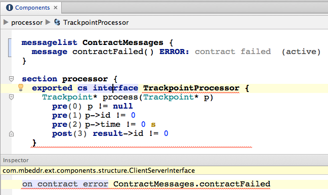
You can now open the inspector for the interface and reference this message from there:
Figure
7.4.1-A: A message definition used in the interface definition to report contract failures.
There are still errors. The first one complains that the message list must be exported if the interface is exported. We fix it by exporting the message list (via an intention). The next error complains that the message needs to have to integer arguments to represent the operation and the pre- or postcondition. We change it thusly (note that there are quick fixes available to adapt the signatures in the required way).
7.4.2 A first Component
We create a new component by typing component. We call it Nuller. It has one provided port called processor that provides the TrackpointProcessor interface.
exported component Nuller extends nothing {
provides TrackpointProcessor processor
} component Nuller
After you add only the provided port, you get an error that complains that the component needs to implement the operations defined by the port's interface; we can get those automatically generated by using a quick fix from the intentions menu on the provided port. This gets us the following:
exported component Nuller extends nothing {
provides TrackpointProcessor processor
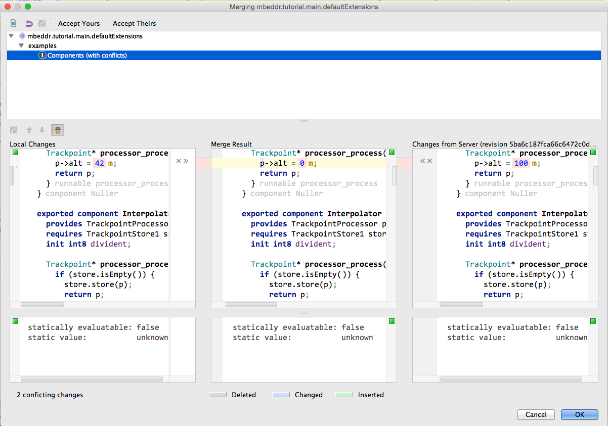
Trackpoint* processor_process(Trackpoint* p) <= op processor.process {
p.alt = 42 m;
return p;
} runnable processor_process
} component Nuller
The processor_process runnable is triggered by an incoming invocation of the process operation defined in the TrackpointProcessor interface. The Nuller simply sets the altitute to zero.
Let us now write a simple test case to check this component. To do that, we first have to create an instance of Nuller. We create an instance configuration that defines exactly one instance of this component. Also, we add an adapter. An adapter makes a provided port of a component instance (Nuller.processor) available to a regular C program under the specified name n:
instances nullerInstancesFailing {

  instance Nuller nuller

  adapt n -> nuller.processor

}
Now we can write a test case that accesses the n adapter -- and through it, the processor port of the Nuller component instance nuller. We create a new Trackpoint, using 0 as the id -- intended to trigger a contract violation (remember pre(1) p->id != 0). To enter the &tp just enter a &, followed by tp.
section testNullerFailing {

  instances nullerInstancesFailing {

  instance Nuller nuller

  adapt n -> nuller.processor

}


  exported testcase testNullerFailing {

  initialize nullerInstancesFailing;

  Trackpoint tp = {

  id = 0,

  time = 0 s,

  alt = 1000 m

};

  n.process(&tp);

  assert(0) tp.alt == 0 m;

} testNullerFailing(test case)

} section testNullerFailing
Before we can run this, we have to make sure that the instances are initialized (cf. the warning you get on them). We do this right in the beginning of the test case. We then create a trackpoint and assert that it is correctly nulled by the Nuller.
section testNullerFailing {

  instances nullerInstancesFailing {

  instance Nuller nuller

  adapt n -> nuller.processor

}


  exported testcase testNullerFailing {

  initialize nullerInstancesFailing;

  Trackpoint tp = {

  id = 0,

  time = 0 s,

  alt = 1000 m

};

  n.process(&tp);

  assert(0) tp.alt == 0 m;

} testNullerFailing(test case)

} section testNullerFailing
To make the system work, you have to import the Components module into the Main module so you can call the testNullerFailing test case from the test expression in Main. In the build configuration, you have to add the missing modules to the executable (using the quick fix). Finally, also in the build configuration, you have to add the components configuration item:
Configuration Items:

  reporting: printf (add labels false)

  physical units (config = Units Declarations (mbeddr.tutorial.main.m1))

  components: no middleware

              wire statically: false
You can now rebuild and run. As a result, you'll get contract failures:
./MbeddrTutorial

$$runningTest: running test () @FunctionPointers:test_testProcessing:0#767515563077315487

$$runningTest: running test () @Components:test_testNuller:0#767515563077315487

$$contractFailed: contract failed (op=0, pc=1) @Components:null:-1#1731059994647588232

$$contractFailed: contract faied (op=0, pc=2) @Components:null:-1#1731059994647588253
We can fix these problems by changing the test data to conform to the contract, i.e.
section testNullerOK {

  instances nullerInstancesOK {

  instance Nuller nuller

  adapt n -> nuller.processor

}


  exported testcase testNullerOK {

  initialize nullerInstancesOK;

  Trackpoint tp = {

  id = 10,

  time = 10 s,

  alt = 100 m

};

  n.process(&tp);

  assert(0) tp.alt == 0 m;

} testNullerOK(test case)

} section testNullerOK
Let us provoke another contract violation by returning from the implementation in the Nuller component a Trackpoint whose id is 0.
Running it again provokes another contract failure. Notice how the contract is specified on the interface, but they are checked for each component implementing the interface. There is no way how an implementation can violate the interface contract without the respective error being reported!
7.4.3 Verifying Contracts Statically
[ToDo:
Need to fill in the static verification part here.
]
7.4.4 Collaborating and Stateful Components
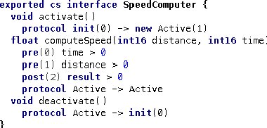
Let us look at interactions between components. We create a new interface, the
TrackpointStore1. It can store and return trackpoints. Here is the basic interface:
exported cs interface TrackpointStore1 {

  void store(Trackpoint* tp)

  Trackpoint* get()

  Trackpoint* take()

  query boolean isEmpty()

}
Let us again think about the semantics: you shouldn't be able to get or take stuff from the store if it is empty, you should not put stuff into it when it is full, etc. These things can be expressed as pre- and postconditions. The following should be pretty self-explaining. The only new thing is the query operation. Queries can be used from inside pre- and postconditions, but cannot modify state
exported cs interface TrackpointStore1 {

  void store(Trackpoint* tp)

  pre(0) isEmpty()

  pre(1) tp != null

  post(2) !isEmpty()

  Trackpoint* get()

  pre(0) !isEmpty()

  Trackpoint* take()

  pre(0) !isEmpty()

  post(1) result != null

  post(2) isEmpty()

  query boolean isEmpty()

}
These pre- and postconditions mostly express a valid sequence of the operation calls: you have to call store before you can call get, etc. This can be expressed directly with protocols, as implemented in TrackpointStore2:
exported cs interface TrackpointStore2 {


  void store(Trackpoint* tp)

  protocol init(0) -> new full(1)


  Trackpoint* get()

  protocol full -> full


  Trackpoint* take()

  post(0) result != null

  protocol full -> init(0)


  query boolean isEmpty()

}
You can add a new protocol using the respective intention. The protocol is essentially a state machine. On each operation you can specify the transition from the old to the new state. We have one special state which is called initial. On a transition you can either jump into an already existing state or create a new state and then directy move into that. I.e. you see on the store operation that we transition from the initial state into the newly created full state. The operation get can now make use of the previously created full state and does not create a new state. It is also worth mentioning that you can reset the protocol by transitioning into the initial state again (as done in take)
The two interfaces are essentially equivalent, and both are checked at runtime and lead to errors if the contract is violated.
We can now implement a component that provides this interface: InMemoryStorage Most of the following code should be easy to understand based on what we have discussed so far. There are two new things. There is a field Trackpoint* storedTP; that represents component state.
Second there is an on-init runnable: this is essentially a constructor that is executed as an instance is created.
void init() <= on init {

  storedTP = null;

  return;

} runnable init
To keep our implementation module Components well structured we can use sections. A section is a named part of the implementation module that has no semantic effect beyond that. Sections can be collapsed.
module Components imports DataStructures {


  exported messagelist ContractMessages {...}


  section processor {...}


  section store {

  	exported cs interface TrackpointStore1 {

    	...

  	}

  	exported cs interface TrackpointStore2 {

    	...

  	}

    exported component InMemoryStorage extends nothing {

	    ...

  	}

  }


  instances nullerInstances {...}

  test case testNuller {...}

  instances interpolatorInstances {...}

  exported test case testInterpolator { ... }

}
We can now implement a second processor, the Interpolator. For subsequent calls of process it computes the average of the two last speeds of the passed trackpoints. Let us start with the test case. Note how p2 has its speed changed to the average of the p1 and p2 originally.
section testInterpolator {
instances interpolatorInstances {
instance InMemoryStorage store
instance Interpolator interpolator(divident = 10)
connect interpolator.store to store.store
adapt ip -> interpolator.processor
}
exported testcase testInterpolator {
initialize interpolatorInstances;
Trackpoint p1 = {
id = 1,
time = 1 s,
speed = 10 mps
};
Trackpoint p2 = {
id = 1,
time = 1 s,
speed = 20 mps
};
ip.process(&p1);
assert(0) p1.speed == 10 mps;
ip.process(&p2);
assert-equals(1) p2.speed == 3 mps;
} testInterpolator(test case)
mock component StorageMock report messages: true {
provides TrackpointStore1 store
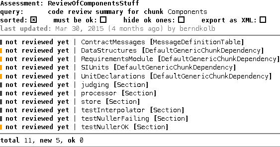
Trackpoint* lastTP;
total no. of calls is 5
sequence {
step 0: store.isEmpty return true;
step 1: store.store {
assert 0: parameter tp: tp != null
}
do { lastTP = tp; }
step 2: store.isEmpty return false;
step 3: store.take return lastTP;
step 4: store.store
}
}
instances interpolatorInstancesWithMock {
instance StorageMock storeMock
instance Interpolator ip(divident = 2)
connect ip.store to storeMock.store
adapt ipMock -> ip.processor
}
exported testcase testInterpolatorWithMock {
initialize interpolatorInstancesWithMock;
Trackpoint p1 = {
id = 1,
time = 1 s,
speed = 10 mps
};
Trackpoint p2 = {
id = 2,
time = 2 s,
speed = 20 mps
};
ipMock.process(&p1);
ipMock.process(&p2);
validatemock(0) interpolatorInstancesWithMock:storeMock;
} testInterpolatorWithMock(test case)
} section testInterpolator
Let us look at the implementation of the Interpolator:
exported component Interpolator extends nothing {

  provides TrackpointProcessor processor

  requires TrackpointStore1 store

  init int8 divident;


  Trackpoint* processor_process(Trackpoint* p) <= op processor.process {

  if (store.isEmpty()) {

  store.store(p);

  return p;

} else {

  Trackpoint* old = store.take();

  p.speed = (p.speed + old.speed) / divident;

  store.store(p);

  return p;

}

} runnable processor_process

} component Interpolator
A few things are worth mentioning. First, the component requires another interface, TrackpointStore1. Any component that implements this interface can be used to fulfil this requirement (we'll discuss how, below). Second, we use an init field. This is a regular field from the perspective of the component (i.e. it can be accessed from within the implementation), but it is special in that a value for it has to be supplied when the component is instantiated. Third, this example shows how to call operations on required ports (store.store(p);). The only remaining step before running the test is to define the instances:
instances interpolatorInstances {

  instance InMemoryStorage store

  instance Interpolator interpolator(divident = 10)

  connect interpolator.store to store.store

  adapt ip -> interpolator.processor

}
A few interesting things. First, notice how we pass in a value for the init field divident as we define an instance of Interpolator. Second, we use connect to connect the required port store of the ipc instance to the store provided port of the store instance. If you don't do this you will get an error on the ipc instance since it requires this thing to be connected (there are also optional required ports which may remain unconnected and multiple required ports which can be connected to more than one required port). Finally, the provided interface processor is made available to other code as the variable ip. You can run the test case now. On my machine here it works successfully :-)
To better understand the connections between component instances, there is also a graphical editor available. To switch to the graphical wireing you can select the respective option form the menu.
7.4.5 Mocks
Let us assume we wanted to test if the Interpolator works correctly with the TrackpointStore interface. Of course, since we have already described the interface contract semantically we would find out quickly if the Interpolator would behave badly. However, we can make such a test more explicit. Let us revisit the test from above:
section testInterpolator {


  instances interpolatorInstances {

  instance InMemoryStorage store

  instance Interpolator interpolator(divident = 10)

  connect interpolator.store to store.store

  adapt ip -> interpolator.processor

}


  exported testcase testInterpolator {

  initialize interpolatorInstances;

  Trackpoint p1 = {

  id = 1,

  time = 1 s,

  speed = 10 mps

};

  Trackpoint p2 = {

  id = 1,

  time = 1 s,

  speed = 20 mps

};

  ip.process(&p1);

  assert(0) p1.speed == 10 mps;

  ip.process(&p2);

  assert-equals(1) p2.speed == 3 mps;


} testInterpolator(test case)


  mock component StorageMock report messages: true {

  provides TrackpointStore1 store

  Trackpoint* lastTP;

  total no. of calls is 5

  sequence {

  step 0: store.isEmpty return true;

  step 1: store.store {

    assert 0: parameter tp: tp != null

  }

  do { lastTP = tp; }

  step 2: store.isEmpty return false;

  step 3: store.take return lastTP;

  step 4: store.store

}

}


  instances interpolatorInstancesWithMock {

  instance StorageMock storeMock

  instance Interpolator ip(divident = 2)

  connect ip.store to storeMock.store

  adapt ipMock -> ip.processor

}


  exported testcase testInterpolatorWithMock {

  initialize interpolatorInstancesWithMock;

  Trackpoint p1 = {

  id = 1,

  time = 1 s,

  speed = 10 mps

};

  Trackpoint p2 = {

  id = 2,

  time = 2 s,

  speed = 20 mps

};

  ipMock.process(&p1);

  ipMock.process(&p2);

  validatemock(0) interpolatorInstancesWithMock:storeMock;

} testInterpolatorWithMock(test case)

} section testInterpolator
In this test, we expect the following: when we call process first, the store is still empty, so the interpolator stores a new trackpoint. When we call process again, we expect the interpolator to call take and then store. In both cases we expect isEmpty to be called first.
We can test for this behavior explicitly via a mock. A mock is a component that specifies the behavior it expects to see on a provided port during a specific test case. The crucial point about mocks is that a mock implements each operation invocation separately (the steps below), whereas a regular component or even a stub just describes each operation with one implementation. This makes a mock implementation much simpler -- it doesn't have to replicate the algorithmic implementation of the real component. Let us look at the implementation:
mock component StorageMock report messages: true {

  provides TrackpointStore1 store

  Trackpoint* lastTP;

  total no. of calls is 5

  sequence {

  step 0: store.isEmpty return true;

  step 1: store.store {

    assert 0: parameter tp: tp != null

  }

  do { lastTP = tp; }

  step 2: store.isEmpty return false;

  step 3: store.take return lastTP;

  step 4: store.store

}

}
This mock component expresses that we expect 5 calls in total. Then we describe the sequence of calls we expect. The first one must be a call to isEmpty and we return true. Then we expect a store, and for the sake of the example, we check that tp is not null. We also store the tp parameter in a field lastTP so we can return it later (you can add the parameter assertions and the do body with intentions). We then expect another isEmpty query, which we now answer with false. At this point we expect a call to take, and another call to store. Notice how we return null from take: this violates the postcondition! However, pre- and postconditions are not checked in mock components because their checking may interfere with the expectations! Also, we have slightly changed the test case so we don't stumble over the null. We don't assert anything about the result of the process calls:
exported testcase testInterpolatorWithMock {

  initialize interpolatorInstancesWithMock;

  Trackpoint p1 = {

  id = 1,

  time = 1 s,

  speed = 10 mps

};

  Trackpoint p2 = {

  id = 2,

  time = 2 s,

  speed = 20 mps

};

  ipMock.process(&p1);

  ipMock.process(&p2);

} testInterpolatorWithMock(test case)
Two more steps are required for this test to work. The first one is the instances and the wiring. Notice how we now connect the interpolator with the mock:
instances interpolatorInstancesWithMock {

  instance StorageMock storeMock

  instance Interpolator ip(divident = 2)

  connect ip.store to storeMock.store

  adapt ipMock -> ip.processor

}
The second thing is the test case itself. Obviously, we want the test case to fail if the mock saw something other than what it expects on its port. We can achieve this by using the validate mock statement in the test:
validatemock(0) interpolatorInstancesWithMock:storeMock;
Check out the complete testInterpolator test case.
7.4.6 Sender/Receiver Interfaces
So far we have always used client/server interfaces to communicate between components. These essentially define a set of operations, plus contracts, that can be invoked in a client/server style. However, mbeddr comes with a second kind of interface, the sender/receiver interface. In this case, the providing and requiring components exchange data items. To demonstrate how they work, let us explore another aspect of the application around Trackpoints (the example is in the ComponentsSRI implementation module). The data has to be collected in the airplane. Let us assume we have the following components:
- a GPS to provide the position
- a speed indicator for the speed
-
a flight recorder, whose job it is to create lists of
Trackpoints that capture the progress of the flight
All these components are time-triggered, i.e. it is assumed that they execute in regular intervals, by some kind of scheduler. They all provide an interface Timed that provides an operation tick that is called by the scheduler. So far, these components don't exchange any data yet: sender/receiver interfaces will be used for that later. Here is the code so far:
module ComponentsSRI imports DataStructures {


  exported cs interface Timed {

    void tick()

  }


  exported component GPS extends nothing {

    provides Timed timed

    void timed_tick() <= op timed.tick {}

  }


  exported component SpeedIndicator extends nothing {

    provides Timed timed

    void timed_tick() <= op timed.tick {}

  }


  exported component FlightRecorder extends nothing {

    provides Timed timed

    void timed_tick() <= op timed.tick {}

  }


}
Let's now look at the data exchange, focussing on the position first. Here is a sender/receiver interface position provider. The interface declares a set of data elements, in this case with physical units:
exported sr interface PositionProvider {

  int8/m/ x;

  int8/m/ y;

  int16/m/ alt;

}
The GPS is supposed to provide this data, so we give it a provided port with this interface:
exported component GPS extends nothing {

  provides PositionProvider pos

  provides Timed timed

  void init() <= on init {

  pos.x = 0 m;

  pos.y = 0 m;

  pos.alt = 0 m;

} runnable init

  void timed_tick() <= op timed.tick {

  pos.x++;

  pos.y++;

} runnable timed_tick

} component GPS
Note how from within component runnables we can use expressions to assign to the data values defined in the interface as if they were normal fields. Let us now look at the flight recorder. It is supposed to read the data written by the GPS (and the same with the speed indicator):
exported component FlightRecorder extends nothing {

  provides Timed timed

  requires PositionProvider pp

  requires SpeedProvider sp

  Trackpoint[1000] recordedFlight;

  uint16 count = 0;

  void timed_tick() <= op timed.tick {


  with (recordedFlight[count]) {

  id = ((int8) count);

  x = pp.x;

  y = pp.y;

  alt = pp.alt;

  speed = sp.speed;

}

  count++;

} runnable timed_tick

  Trackpoint getFlightNo(uint16 no) <= no trigger {

  return recordedFlight[no];

} runnable getFlightNo

} component FlightRecorder
Inside the with-statement, we can access the data acquired via the pp and sp required ports. What distinguishes this from global variables, of course, is that the component instances still have to be wired: required ports have to be connected to provided ports, in this case, defining access to the data items:
instances instances {

  instance GPS gps_comp

  instance SpeedIndicator indicator

  instance FlightRecorder recorder

  connect recorder.sp to indicator.speed

  connect recorder.pp to gps_comp.pos

  adapt gps -> gps_comp.timed

  adapt si -> indicator.timed

  adapt rec -> recorder.timed

}
This part of the tutorial only provided a few examples of Interfaces and Components. For a full discussion of Interfaces and Components see \\fordetails{Interfaces and Components}{\\sect{details_components}}
7.4.7 Composite Components
Components are great to structure your code in reusable pieces. But typically when your systems grow you want to reuse whole subsystems. To the outside they look exactly like any other component but on the inside they again are wired up out of many components. This can be achieved with mbeddr's composite components.
A composite component, as any other component can require and provide interfaces from/to its environment. In addition to regular components it has an additional code block called internal instances for instantiating other components and wire them up.
Let's build an imaginary GPS parser that can be reused. The first interface we create is a client server interface which accepts single characters. Those characters will be used by a line parser which can tokenize the stream of chars into whole lines and at the same time figures out which command was send by the client. Each line is then fed into another component which itself delegates the command to a command handler. This command handler parses the command and transforms the data into a struct that can be easily consumed by a client. The client of the GPS parser does not need to know how the parsing works internally and that it again is split up into separate components. The only relevant part is that she needs to provide the system with the stream of characters and takes the events produced by the GPS parser to work on them. To achieve this we create a composite component which provides the CharParser and requires the NmeaRmcEventProcessor. In the wiring we instantiate the respective components and wire them up. Finally, we delegate the outside required and provided ports. The whole code for the composite component is here. Don't forget to add the composite components config item to the build configuration.
exported composite component NmeaStack {


  provides CharParser charParser

  requires NmeaRmcEventProcessor rmcEventProcessor


  internal instances {

  instance NmeaLineParserImpl lineParser

  instance NmeaSentenceHandlerImpl sentenceHandler


  instance NmeaRmcHandlerImpl rmcHandler

  connect lineParser.sentenceHandler to sentenceHandler.sentenceHandler

  connect multi sentenceHandler.commandHandlers to rmcHandler.nmeaCommandHandler


  delegate charParser to lineParser.charParser

  delegate rmcEventProcessor to rmcHandler.nmeaRmcEventProcessor

}

}
7.4.8 Interface Types
In a few rare cases you want to store a required port also as a local variable (e.g. when iterating over a bunch of multiports where you filter out some of them). In even rarer cases you may want to pass a required port as an argument to a function or runnable you are calling or store it in a global variable. To address those use cases we introduces a type in mbeddr called interface. In order to use an interface in such a interface type this interface has to be specially marked with an annotation .
exported cs interface NmeaCommandHandler can be used as type {

  boolean canHandle(string command)

  void handle(int8[MAX_NMEA_WORD_COUNT]* words, uint8 wordCount)

}
void sentenceHandler_parseSentence(int8[MAX_NMEA_WORD_COUNT]* words, uint8 wordCount) <= op sentenceHandler.parseSentence {

  interface<NmeaCommandHandler> handlerToCall = null;

  for (i ++ in [0..MAX_NMEA_COMMAND_HANDLER_COUNT[) {

  if (commandHandlers[i] != null && commandHandlers[i].canHandle(words[0])) {

  handlerToCall = commandHandlers[i];

} if

} for

  handlerToCall.handle(words, wordCount);

} runnable sentenceHandler_parseSentence
The example above actually would not need the interface type as the handle runnable could be called right in place.
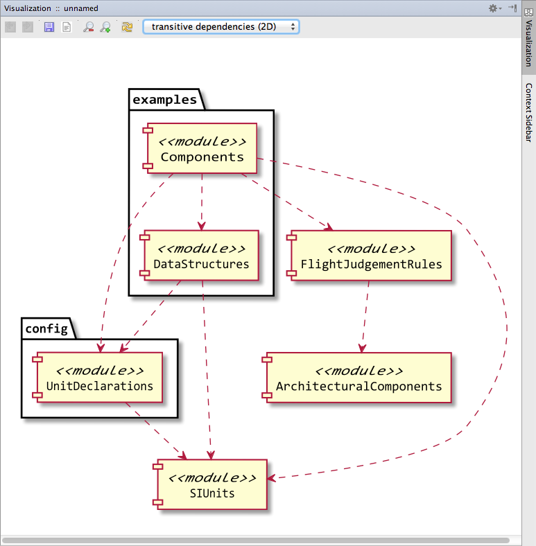
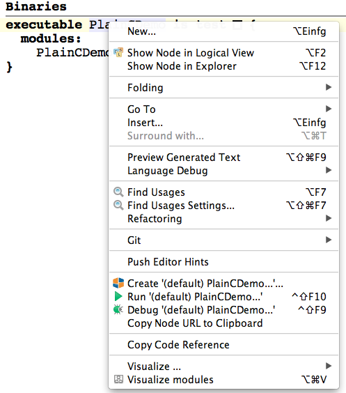
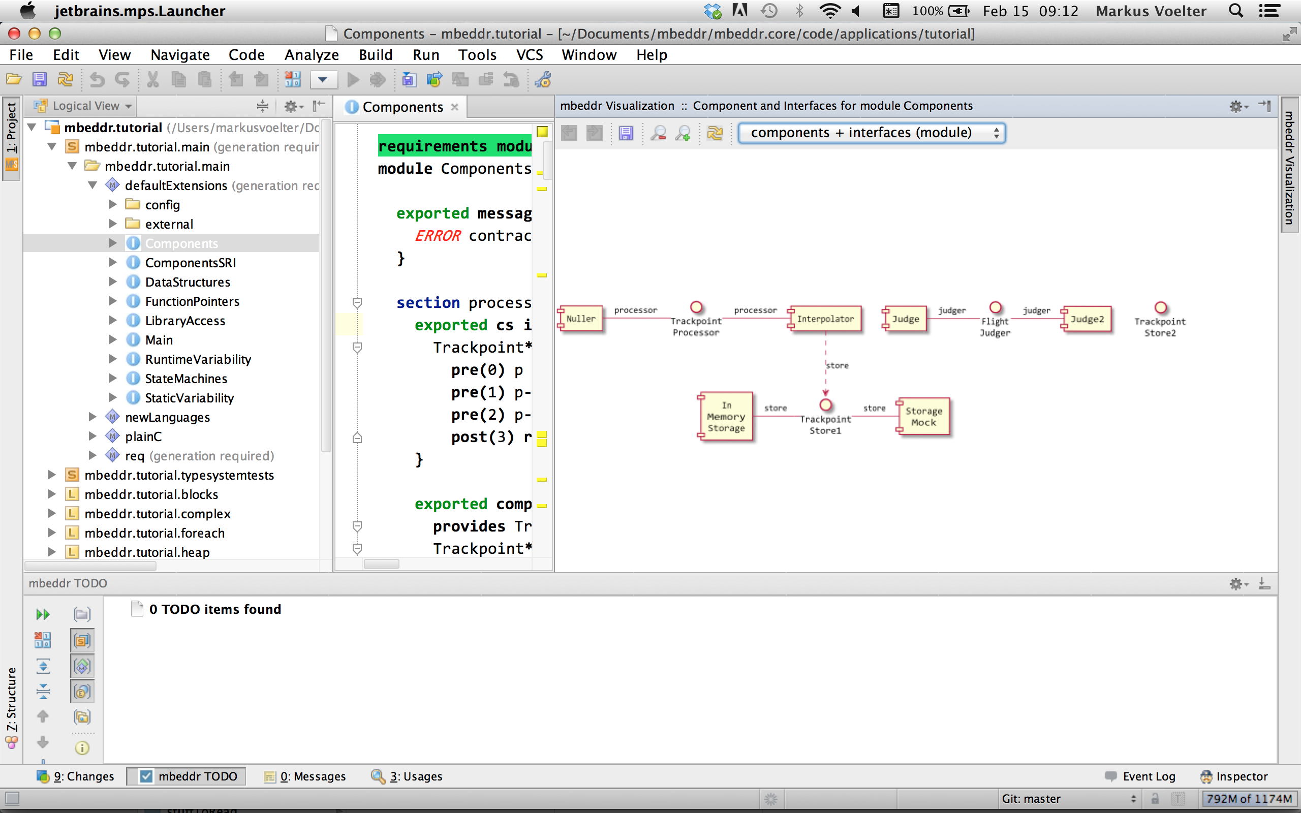
7.4.9 Visualizing Components
mbeddr's diagramming capabilities are put to use in two ways in the context of components: component/interface dependencies and instance diagrams.
* Component/Interface Dependencies Select a component or an interface and execute the Visualize action from the context menu (or press Ctrl+Alt+V). Fig. 7.4.9-A shows the result.
Figure
7.4.9-A: The interface/components dependency diagram shows all components visible from the current module, the interfaces, and the provided (solid lines) and required ports (dashed lines).
* Instance/Wiring Diagrams You can also select an instance configuration and visualize it. You'll get a diagram that shows component instances and their connections (Fig. 7.4.9-B).
Figure
7.4.9-B: This diagram shows component instances and their connectors. The label in the instance boxes contain the instance name and the component name (after the colon). The edges represent connectors. The label shows the required port (before the arrow, the provided port name (after the arrow), and the name of the interface used by the two ports (on the new line).
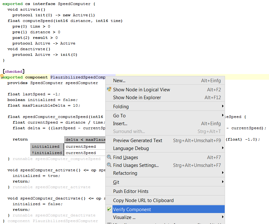
7.4.10 Contract Verification
mbeddr comes with support for verifying contracts of components statically. This verification is based on C-level verification with CBMC (for a more detailed discussion about the formal verification with mbeddr, please look at Section Functional Verification. Let's set up our tutorial to use verification. Let us verify the InMemoryStorage component. To do so, first add the com.mbeddr.analyses.componentcontracts devkit to the model that contains the components code. Then use an intention to add the verifiable flag to the component. To make the verification work, you will have to provide some more information in the inspector:
entry point: verification

  loops unwinding: 2

  unwinding assertions: false
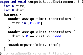
Let us look at the three parameters you have to set here: The first one determines from where the program is "executed". The entry point should be selected to be "close" to the to-be-verified component (if you verify the whole system, then, at least for big systems, this will take long). In our case we use a special test case verification, which looks as follows:
instances verificationInstances {

  instance Interpolator interpol(divident = 2)

  connect interpol.store to store.store

  instance InMemoryStorage store

  adapt verificationInterpolator -> interpol.processor

}
exported testcase verification {

  initialize verificationInstances;

  Trackpoint p1 = {

  id = 1,

  time = 1 s,

  speed = 10 mps

};

  Trackpoint p2 = {

  id = 1,

  time = 1 s,

  speed = 20 mps

};

  verificationInterpolator.process(&p1);

  verificationInterpolator.process(&p2);

} verification(test case)
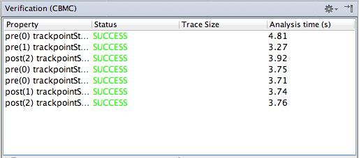
The second line in the configuration determines how often a loop is executed. You should start with low numbers to keep verification times low. Finally, the third parameter determines if the verification should fail in case it cannot be proven that the unwinding loops number is sufficient. You can now run the verification by selecting the component and executing the action. After a few seconds, you'll get a result table that reports everything as ok (see Fig. 7.4.10-A): every precondition of every operation in every provided port has been proven to be correct.
Figure
7.4.10-A: The table that shows the verification results; everything is ok in this case.
Let us introduce an error. The following version of the trackpointStore_store runnable does not actually store the trackpoint. This violates the postcondition, which claims that storedTP != null. Note that for the analysis to work, all paths through the body of a function (or a runnable) must end with a return (you'll get an in-IDE error if you don't do this).
void trackpointStore_store(Trackpoint* tp) <- op store.store {

  return;

}
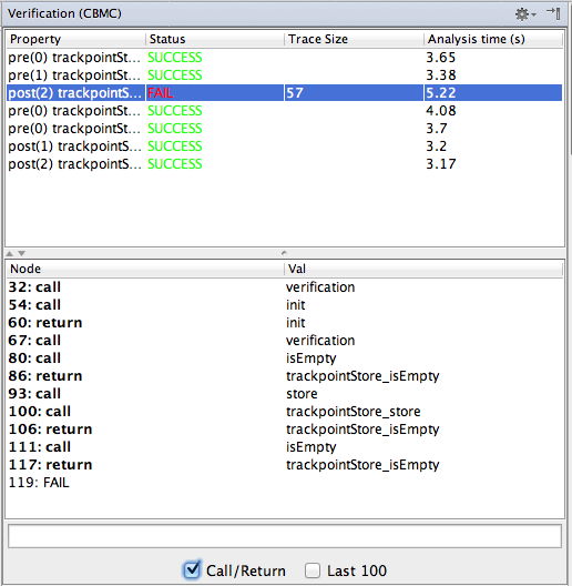
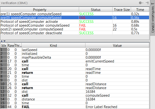
Let us rerun the verification. Now we get an error, as shown in Fig. 7.4.10-B. Note how the lower part of the table now shows the execution trace that led to the contract violation. You should check the Call/Return checkbox to filter the trace to only show the call/return-granularity, and not every statement. You can also double-click onto the trace elements to select the particular program element in the code.
Figure
7.4.10-B: The table that shows the verification results; now we have an error, and the trace in the bottom half shows an example execution that led to the error.
7.5 Decision Tables
Let us implement another interface, one that lets us judge flights (we do this in a new section in the Components module). The idea is that clients add trackpoints, and the FlightJudger computes some kind of score from it (consider some kind of biking/flying competition as a context):
exported cs interface FlightJudger {

  void reset()

  void addTrackpoint(Trackpoint* tp)

  int16 getResult()

}
Here is the basic implementation of a component that provides this interface.
exported component Judge extends nothing {

  provides FlightJudger judger

  int16 points = 0;

  void judger_reset() <- op judger.reset {

    points = 0;

  }

  void judger_addTrackpoint(Trackpoint* tp) <- op judger.addTrackpoint {

    points += 0; // to be changed

  }

  int16 judger_getResult() <- op judger.getResult {

    return points;

  }

}
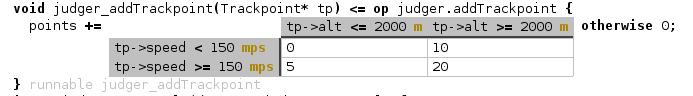
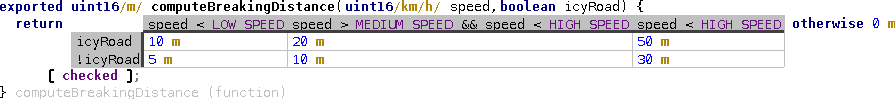
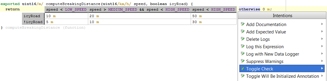
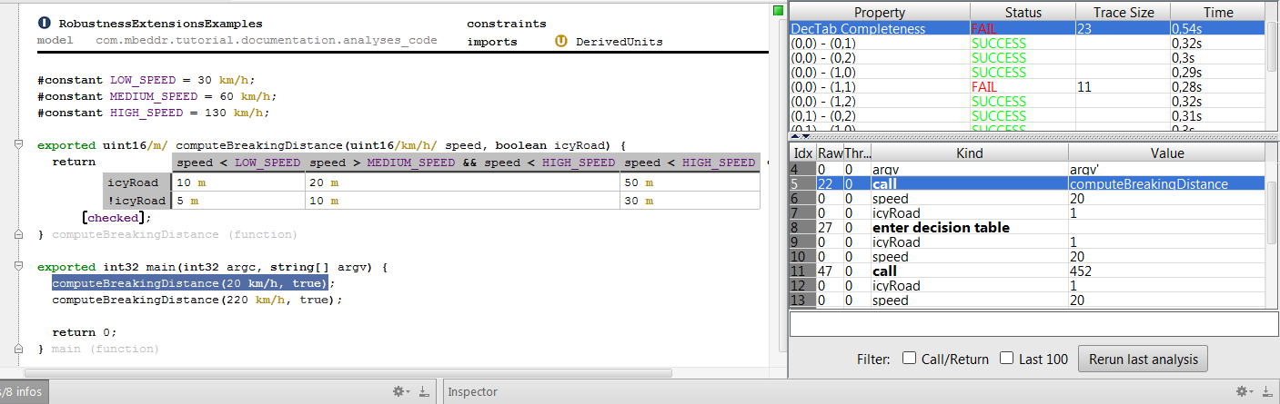
Of course the implementation of addTrackpoint that just adds 0 to the points doesn't make much sense yet. The amount of points added should depend on how fast and how high the plane (or whatever) was going. The following screenshot shows an embedded decision table that computes points (Notice we mix the components language, the decision tables and the units in one integrated program):
You can create the decision on your own by first of all typing the keyword dectab - this instanciates the concept. To add a column, hit enter in one of the cells. For adding a row, move your cursor on the left side of the table (between the default return value and the table) and hit enter. Now, let us write a test. Of course we first need an instance of Judge:
instances instancesJudging {

  instance Judge theJudge

  adapt j -> theJudge.judger

}
Below is the test case. It contains two things you maybe haven't seen before. There is a second form of the for statement that iterates over a range of values. The range can be exclusive the ends or inclusive (to be changed via an intention). In the example we iterate from 0 to 4, since 5 is excluded. The introduceunit construct can be used to "sneak in" a unit into a regular value. This is useful for interacting with non-unit-aware (library) code. Note how the expression for speed is a way of expressing the same thing without the introduceunit in this case. Any expression can be surrounded by introduceunit via an intention.
exported testcase testJudging {

  initialize instancesJudging;

  j.reset();

  Trackpoint[5] points;

  for (i ++ in [0..5[) {

  points[i].id = ((int8) i);

  points[i].alt = 1810 + 100 * i m;

  points[i].speed = 130 mps+ 10 mps* i;

  j.addTrackpoint(&points[i]);

} for

  assert-equals(0) j.getResult() == 0 + 0 + 20 + 20 + 20;

} testJudging(test case)
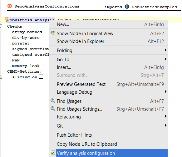
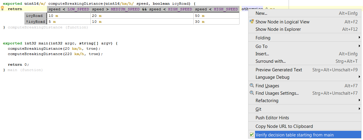
7.5.1 Verifying the Decision Table
So far so good. The test case is fine. However, as with many tests, this one only tests part of the overall functionality. And in fact, you may have noticed that an error lurks inside our decision table: for 2000 m of altitude, the table is non-deterministic: both conditions in the column header work! We could find this problem with more tests, or we could use formal verification as described in Section Checking Decision Tables.